Computer Practicum 2
This computer practicum contains the following four parts:
Learning objectives
After this computer practicum the student should be able to do the following in R Commander:
Plot and interpret the Binomial distribution;
Determine probabilities from the Binomial distribution;
Perform a simulation using a Binomial situation;
Produce and interpret a plot of a normal distribution;
Determine probabilities from a normal distribution;
Indicate tail probabilities;
Identify estimates for the (population) mean \(\mu\) and (population) standard deviation \(\sigma\);
Make a Q-Q plot.
Part 1 - Binomial Distribution
The following questions are related to the binomial distribution. Use R Commander to answer the questions. Use the answer sheet, that is handed out by the teacher, to write down your answers.
You can use the following information to answer questions a) to g):
When rolling a fair die, the probability of obtaining the outcome \(6\) equals \(\frac{1}{6} \approx 0.1667\). Assume the fair die is rolled five \((n = 5)\) times, and let \(y\) be the number of times obtaining the outcome \(6\) in \(5\) rolls of a fair die. Then \(y \sim \mbox{Bin}(n = 5,\ \pi = \frac{1}{6})\).
- Visualize the binomial distribution mentioned above; \(\mbox{Bin}(n = 5,\ \pi = \frac{1}{6})\). Go to: Distributions > Discrete distributions > Binomial distribution > Plot binomial distribution\(\ldots\) Use for Probability of success: \(0.1667\) and provide the desired \(n\) in the field behind Binomial trials. Make a sketch of the graph on the answering form.
The resulting graph will be displayed in a separate R Graphics window:
If necessary resize the window to see all text of the title above the binomial distribution!
On the \(x\)-axis the Number of successes \(5\) is not included, because this probability is extremely small. However, \(5\) times obtaining the outcome \(6\) out of \(5\) rolls of a fair die is a possibility even when the probability is extremely small.
-
Calculate the probability of obtaining \(0\) times the outcome six in \(5\) rolls of the fair die. Go to: Distributions > Discrete distributions > Binomial distribution > Binomial probabilities\(\ldots\) The probabilities for each number of successes, \(P(y = k)\ \forall\ k \in \{0,1,\ldots,5\}\), are shown in the part Output of the R Commander window. After you have found the answer in the part Output of the R Commander window and have filled in the answer on the form, try to get the same answer:
from the graph you have made under a).
using your graphing calculator (if you have one).
-
Calculate the probability of obtaining \(3\) times the outcome six in \(5\) rolls of the fair die. After you have found the answer in the part Output of the R Commander window and have filled in the answer on the form, try to get the same answer:
from the graph you have made under a).
using your graphing calculator (if you have one).
-
Calculate the probability of obtaining at most \(1\) time the outcome six in \(5\) rolls of the fair die. Go to: Distributions > Discrete distributions > Binomial distribution > Binomial tail probabilities\(\ldots\) Fill the fields behind Variable value(s), Binomial trials, Probability of success with the appropriate values and select the appropriate tail for the calculation. After you have found the answer in the part Output of the R Commander window and have filled in the answer on the form, try to get the same answer:
from the graph you have made under a).
using your graphing calculator (if you have one).
Determine the probability of obtaining at least \(2\) times the outcome six in \(5\) rolls of the fair die by using the answer of d) and the complement rule. When you have found the answer, try also to find the answer by using R Commander.
When selecting the Upper tail in probability calculations, R Commander (and R in general) calculates \(P(y > k)\) and not \(P(y \geq k)\). Think carefully, what you should enter in the field behind Variable value(s), which represents \(k\), to get the correct answer.

-
Simulate \(500\) times rolling a fair die \(5\) times and counting the number of times of obtaining the outcome six. Go to: Distributions > Discrete distributions > Binomial distribution > Sample from binomial distribution\(\ldots\), use the settings shown in Figure 1 and click the OK button to execute. Next:
Have a look at the created data object “BinomialSamples”, using View data set.
Calculate the mean of the variable “
obs” with R Commander (calculating the mean of a variable in R Commander was a topic in Computer Practicum \(1\)).Calculate the (population) mean (or expected value) for the number of times obtaining the outcome six in \(5\) rolls with a fair die, as discussed in Tutorial 3.
Use the table in your answer form to calculate the same answer as above in 3. Hint: fill the table using the output created in question b).
- Are the three answers in 2., 3., and 4. exactly the same? Comparable? Can you explain why / who not?
R Commander can be used as a (statistical) calculator. Try it:
- Type on a new line in the R Script part of the R Commander window:
100 * 0.256(keep the blinking cursor on the same line) - Press the Submit button situated on the right side between the R Script and Output part in the R Commander window
- The answer will appear in the Output part of the R Commander window
- Plot the simulated results. Go to: Graphs > Plot discrete numeric variable\(\ldots\), because of the contents of the “
BinomialSamples” object R Commander does not allow making a bar graph. Compare the resulting plot with the plot made in Part 1 a), and explain similarities / differences.
Part 2 - Normal Distribution
The following questions are related to the Normal Distribution. Use R Commander to answer the questions.
- Determine \(P(y > 12)\), when it is given that \(y \sim \mbox{N}(\mu = 12,\ \sigma =5)\). Go to: Distributions > Continuous distributions > Normal distribution > Normal probabilities\(\ldots\) Fill the fields Variable value(s): \(12\), Mean: \(12\), Standard deviation: \(5\), and choose Upper tail by switching the radio button. Click the OK button to execute.
Try to understand, what the filled numbers mean with respect to the asked probability, and why to use Upper tail.
Determine \(P(y < 10) \rightarrow y \sim \mbox{N}(12,\ 5)\).
Give the 95th percentile of the distribution \(y \sim \mbox{N}(12,\ 5)\). Go to: Distributions > Continuous distributions > Normal distribution > Normal quantiles\(\ldots\).
Give the 95^th percentile of the distribution \(x \sim \mbox{N}(0,\ 1)\) (Standard Normal Distribution).
Use the answer of d) to determine the 5th percentile of the distribution \(x \sim \mbox{N}(0,\ 1)\).
Use the following information to answer questions f) to i):
Assume that the height of a random male student (\(y\)) is normally distributed with expected value \(\mu = 182\) and standard deviation \(\sigma = 7\) (cm).
Display a graphical representation of this normal distribution. Go to: Distributions > Continuous distributions > Normal distribution > Plot normal distribution\(\ldots\)
Calculate the probability of a student being taller than \(190\) cm.
Make a visualization of the probability of question f. Go to: Distributions > Continuous distributions > Normal distribution > Plot normal distribution\(\ldots\) and fill in the numbers like as given in the screenshot shown in Figure 2. By clicking behind color on “
#BEBEBE”, the color of the area below the density function can be changed.

- Calculate the probability, that a student is deviating more than one standard deviation from the (population) mean (or expected) height of a male student.
- Make a visualization of the probability of Part 2 Question i). Color the probability in the left-tail green (“
#00FF00”) and in the right-tail orange (“#FFA500”).
Region 1: from \(\ldots\) to \(\ldots\), and Region 2: from \(\ldots\) to \(\ldots\) should be read from left to right.
Therefore, for the green left-tail fill Region 1: from \(0\) to \(\ldots\) (specify your upper boundary).
For the orange right-tail fill Region 2: from \(\ldots\) to \(1000\) (specify your lower boundary).
Part 3 - Estimators and estimates for \(\mu\), and \(\sigma\)
A machine fills packages with sugar. The probability distribution of the weight \(y\) of a random pack of sugar is a normal distribution with mean \(\mbox{E}(y) = \mu_y\) and variance \(\mbox{var}(y) = \sigma_y^2\). To estimate the parameter \(\mu_y\), 10 packs of sugar are selected randomly from the production line and weighed (in g).
The weights are as follows: \(510,\ 525,\ 560,\ 515,\ 455,\ 465,\ 510,\ 505,\ 540,\ 485\).
-
Create a new data set in R Commander by going to: Data > New data set\(\ldots\):
Give it a sensible name, e.g., “
sugar_packages”.Next click the Add row button to get \(10\) rows in the data set.
Click the field labeled “
V1” and enter a sensible variable name (e.g., “weight”).Enter the weights of the randomly selected packages of sugar, and finally click the OK button to create the data set.
Use R Commander to calculate the (sample) mean and (sample) standard deviation.
Statistics > Summaries > Numerical Summaries\(\ldots\) allows for selection of the numerical summary values to calculate on the tab Statistics. Tick or untick the boxes in front of the numerical summary value you want to select or remove.
Fill in the sentence on the answer sheet regarding the (sample) mean \(\bar{y}\), by circling the correct answers.
Fill in the sentence on the answer sheet regarding the (sample) standard deviation \(s\), by circling the correct answers.
Make a Q-Q plot, and judge whether the normality assumption for the weights of randomly selected sugar packages holds here. Go to: Graphs > Quantile-comparison plot\(\ldots\), and click the OK button to create the plot.
Part 4 - Binomial Distribution: Testing a hypothesis with predatory mites
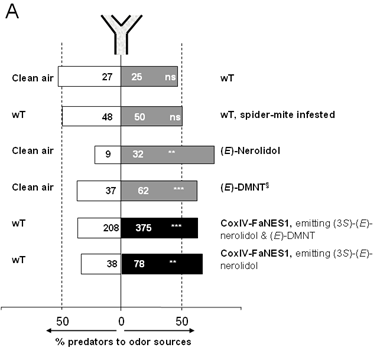
Figure 3 is taken from an article in Science authored by the Laboratory of Entomology at Wageningen University & Research on odorous substances to attract predatory mites to Arabidopsis thaliana plants (commonly known as thale cress, mouse-ear cress, or arabidopsis).
The figure presents the results of six different experiments with an olfactometer, or Y-shaped tube (as shown at the top in Figure 3). The upper ‘bar’ (in Figure 3) represents an experiment in which, for each predatory mite, clean air was blown into one end and air with volatiles from a specific plant (in this case wild Type, or wT thale cress) into the other end. A total of \(52\) predatory mites walked upwards to the end of the olfactometer; \(27\) mites preferred clean air and \(25\) air with volatiles from the wT thale cress plant. This outcome appeared to be non-significant (ns as indicated in the ‘bar’ of the experiment).
In this part of the computer practicum use R Commander to take a closer look at the outcomes of a part of the thale cress experiments presented in Figure 3. Denote the answers on the anwser form, handed to you by your computer practicals teacher.
Experiment comparing Clean air to (E)-Nerolidol
Note that this is the third bar from the top in Figure 3
Let parameter \(\pi\) be the probability, that a predatory mite chooses the odorous substance (E)-nerolidol. The researchers wish to show that predatory mites are attracted by the odorous substance (E)-nerolidol.
Suppose that the mites are not attracted by the odorous substance: what proportion of mites are expected to walk to the end of the Y-shaped tube with the odorous substance (E)-nerolidol?
If the mites are attracted by the odorous substance (E)-nerolidol, do you expect the proportion you mentioned under a) to be higher of lower, or can it be either one of them?
Given your answers to a) and b) formulate the hypothesis of the researchers (i.e., what the researchers wish to show) in terms of population proportions.
What is the probability distribution of the number of mites, that choose for the odorous substance, under the assumption that predatory mites do not have a preference? Denote your answer in the form: \(y \sim \ldots\).
How many predatory mites (out of the \(41\) used in this experiment) are expected to choose air with the odorous substance, when predatory mites do not have a preference?
Do you expect a higher or a lower number of predatory mites to choose the odorous substance, when predatory mites do have a preference?
How many mites eventually did choose the odorous substance in this experiment? In other words: how many ‘successes’ (\(= y\)) were actually observed?
According to Figure 3, the p-value is significant (**: p-value \(< 0.01\)). The p-value will be discussed in an upcoming tutorial, but here it is the probability to observe at least the number of successes as in answer g), when the predatory mites do not have a preference. Use R Commander to calculate this probability (i.e., the p-value). When using Upper tail, remember that R Commander calculates \(P(y > k)\) (where \(k\) represents the number of successes).
Beforehand the researchers wanted to have a probability (here the p-value) of 0.05 or smaller, in order to state that it was proven that mites have a preference for the odorous substance (E)-nerolidol. Give your conclusion based on the probability you have found.
The questions, just answered, are actually hypothesis testing. In upcoming tutorials hypothesis testing will discussed in more detail, including all associated terms and concepts. The questions of Part 4 can be considered as a preview or an ‘amuse’ of what is about to follow.