Tutorial 10

Learning objectives

After this tutorial the student should be able to:

recognize a situation and research question for which a simple linear regression is the appropriate analysis;
mention and explain in own words the five model assumptions of the simple linear regression model;
give the model equation;
mention and use the associated terms (i.e., \(y\), \(x\), \(\beta_0\), \(\beta_1\), \(\sigma\) and \(\varepsilon\)) appropriately;
give the least square estimators for the three model parameters (\(\beta_0\), \(\beta_1\), \(\sigma\));
interpret a scatter plot and regression line;
interpret the regression coefficients;
give (based on R/R Commander output) the estimated regression model;
give (based on R/R Commander output) the estimated \(\sigma\):
apply (based on R/R Commander output) the omnibus \(F\)-test for the model.

Pre-class activity

Watch:

‘Statistics Motivation Clip Landscape Architecture and Spatial Planning’ (Duration: 3:36 min.)

The clip is linked on Brightspace.

Simple Linear Regression

Read:

O&L 7^th Edition:
- paragraph 11.1 pp.555-559 up to smoothers,
- paragraph 11.2 pp.564-568 up to and including Example 11.2, or
O&L 6^th Edition:
- paragraph 11.1 pp.572-576 up to smoothers,
- paragraph 11.2 pp. 581-585 up to and including Example 11.2.

The Simple Linear Regression Model

Model: \(\mbox{E}(y) = \beta_0 + \beta_1 \times x\), or \(y = \beta_0 + \beta_1 \times x + \varepsilon\) with \(\mbox{E}(\varepsilon) = 0\).

Assumptions:

Both \(y\) and \(x\) are quantitative variables.
There is a linear relationship between \(y\) and \(x:\ \mu_y= \beta_0 + \beta_1 \times x\).
\(\mbox{var}(\varepsilon) = \sigma_{\varepsilon}^2\), so \(\mbox{var}(\varepsilon)\) does not depend on the value of \(x\).
The observations \(y_1, y_2,\ldots,\ y_n\) are independent, or equivalently the residuals \(\varepsilon_1,\ \varepsilon_2,\ldots,\ \varepsilon_n\) are independent.
\(\varepsilon_1,\ \varepsilon_2,\ldots,\ \varepsilon_n\) are normally distribution with a population mean (or expected value) \(0\) and constant variance \(\sigma_{\varepsilon}^2\).

Least Squares estimators for the slope and the intercept:

slope \(\hat{\beta}_1 = \frac{\sum (x_i - \bar{x}) (y_i - \bar{y})}{\sum (x_i - \bar{x})^2}\) or \(\hat{\beta}_1 = r_{xy} \times \frac{s_y}{s_x}\)
intercept \(\hat{\beta}_0 = \bar{y} - \hat{\beta}_1 \times \bar{x}\)
The least squares estimators \(\hat{\beta}_0\) and \(\hat{\beta}_1\) are unbiased and they are the best linear unbiased estimators for \(\beta_0\) and \(\beta_1\).

Least Squares estimator for the residual variance

\(\hat{\sigma}^2_{\varepsilon} = s_{\varepsilon}^2 = \frac{\sum(y_i - \hat{y})^2}{n-2}\), where \(\hat{\sigma}^2_{\varepsilon}\) is an unbiased estimator for \(\sigma^2_{\varepsilon}\) (the residual variance).

Remarks about the simple linear regression.

There is no need to calculate the estimates \(\hat{\beta}_0\), \(\hat{\beta}_1\) and \(\hat{\sigma}^2_{\varepsilon}\) by hand. For this the R/R Commander output will be used.
The estimated regression line always passes through the center of all data points \((\bar{x}, \bar{y})\).
The book (O&L) uses the term standard error of estimate for \(\hat{\sigma}_{\varepsilon}\), whereas R/R Commander uses the term Residual standard error. These terms are confusing, because “standard error of estimate” is generally reserved for the precision of an unbiased estimator.

Hypothesis test for the model \(y = \beta_0 + \beta_1 \times x + \varepsilon\) (omnibus \(F\)-test)

Under the assumptions given above:

Null hypothesis \(\mbox{H}_0:\ \beta_1 = 0\) versus \(\mbox{H}_{\mbox{a}}:\ \beta_1 \ne 0\) (i.e., the alternative hypothesis states that the model has predictive value.)
Test statistic (T.S.): \(F = \frac{\mbox{MS}_{\mbox{regression}}}{\mbox{MS}_{\mbox{residual}}}\)
Under \(\mbox{H}_0\) T.S. \(F\) follows a \(F\)-distribution with for the numerator \(1\), and for the denominator \(n - 2\) degrees of freedom.

etc.

Remarks about the hypothesis test fot the model.

The \(F\)-test above is only used for \(\mbox{H}_{\mbox{a}}:\ \beta_1 \neq 0\) (and not for \(\mbox{H}_{\mbox{a}}:\ \beta_1 > 0\) or \(\mbox{H}_{\mbox{a}}:\ \beta_1 < 0\), or any test value other than \(0\)), and is within the frame work of simple linear regression for a straight line equivalent to the \(t\)-test for \(\mbox{H}_{\mbox{a}}:\ \beta_1 \neq 0\) (as will be explained in Tutorial 11).
The \(F\)-test above is only used for a two-tailed alternative hypothesis \(\mbox{H}_{\mbox{a}}: \beta_1 \neq 0\). However, the rejection region is (due to the characteristics of the \(F\)-distribution) always right-tailed. Therefore, the p-value equals \(P(F \geq \mbox{outcome test statistic})\).

Exercises to be done during the tutorial

Exercise 10.1 and Exercise 10.2 are in the presentation handouts of Tutorial 10. Check Brightspace for answers/feedback.

Exercise 10.1

Based on the research of Ruben Dijkhof (MSc Thesis Landscape Architecture and Spatial Planning, see clip linked on Brightspace).

Research Question: What is the effect of the distance to the national ecological network \((x)\), measured in kilometers, on the price of agricultural land \((y)\) in the province Limburg?

It is assumed that \(\mu_y\) and \(x\) are linearly related.

Write down the (mathematical) model and describe all used symbols.

Exercise 10.2

Part of the linear model summary for the Rhizotron potato example:

Coefficients:
             Estimate Std. Error t value Pr(>|t|)    
(Intercept)  5.027743   4.769476   1.054     0.34    
thermal_time 0.088391   0.007811  11.316 9.42e-05 ***
---
Signif. codes:  0 ‘***’ 0.001 ‘**’ 0.01 ‘*’ 0.05 ‘.’ 0.1 ‘ ’ 1

Residual standard error: 7.364 on 5 degrees of freedom
Multiple R-squared:  0.9624,    Adjusted R-squared:  0.9549 
F-statistic: 128.1 on 1 and 5 DF,  p-value: 9.422e-05

Using the partial R/R Commander output above:

a. Provide the equation for the estimated model of the root depth explained by thermal time.

b. Provide an estimate for the (population) mean root depth, when the thermal time equals 0.

c. Provide an estimate for the (population) mean root depth, when the thermal time equals 1.

d. What will be the estimated effect on the (population) mean root depth, when the thermal time increases with 4 degree days?

e. Is there any evidence that the model for root depth explained by thermal time has predictive value?

Post-class activity

Watch:

‘Statistics Motivation Clip Landscape Architecture and Spatial Planning’ (Duration: 3:36 min.), when not done as pre-class activity.

The clip is linked on Brightspace.

Exercises to be done after the tutorial

For answers/feedback check Brightspace.

Exercise 10.3

Based on:

Example 11.2 O&L 7^th Edition pp.566-568, or
Example 11.2 O&L 6^th Edition pp.583-585

Read the introduction of this example (not the questions below it). Use the R/R Commander output below to answer the following questions:

Scatter plots

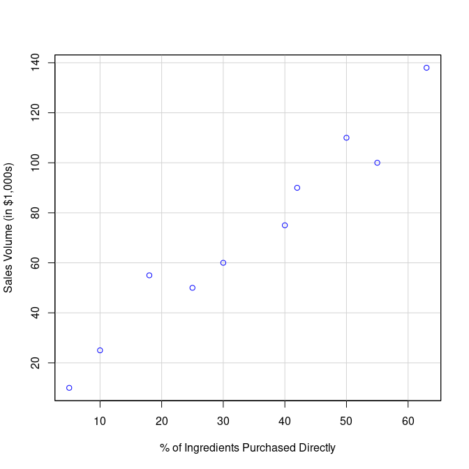
Summary Simple Linear Regression model (straight line model)

Call:
lm(formula = Sales_Volume ~ Purchased_Directly, data = example11_2)

Residuals:
    Min      1Q  Median      3Q     Max 
-13.074  -4.403  -1.607   5.719  14.834 

Coefficients:
                 Estimate Std. Error t value Pr(>|t|)
(Intercept)        4.6979     5.9520   0.789    0.453
Purchased_Directly 1.9705     0.1545  12.750 1.35e-06 ***
---
Signif. codes:  0 ‘***’ 0.001 ‘**’ 0.01 ‘*’ 0.05 ‘.’ 0.1 ‘ ’ 1

Residual standard error: 9.022 on 8 degrees of freedom
Multiple R-squared:  0.9531,    Adjusted R-squared:  0.9472 
F-statistic: 162.6 on 1 and 8 DF,  p-value: 1.349e-06

a. What is the research question in example 11.2?

b. Have a look at the provided scatter plots. What can you read from these plots with respect to the strength of the linear relationship?

c. Give, based on the description of the example in the book, the Simple Linear Regression model (straight line model) and describe all symbols used in terms of the actual problem.

d. Test (\(\alpha = 0.05\)) whether the model has any predictive value. Mention all 8 steps.

e. Is the test performed in d. suitable for the research question (answer a.)? Give arguments.

f. Give the estimated simple linear regression model (straight line model) as an equation.

Exercise 10.4

In a study conducted to examine the quality of fish after 7 days of storage on ice, ten raw fish of the same kind and approximately the same size were caught and prepared for storage on ice. Two of the fish were placed in storage immediately after being caught, two were placed in storage 3 hours after being caught, and two each were placed in storage at 6, 9 and 12 hours after being caught.

Let \(y\) denote a measurement of fish quality (on a 10-point scale) after 7 days of storage on ice, and let \(x\) denote the time after being caught that the fish were placed in storage on ice. The sample data are (see Table 1):

Table 1: Fish quality data

y	x
8.5	0
8.4	0
7.9	3
8.1	3
7.8	6
7.6	6
7.3	9
7.0	9
6.8	12
6.7	12

The following model is assumed: \(y_i = \beta_0 + \beta_1 \times x_i + \varepsilon_i\)

Furthermore assume that the residuals are independent and normally distributed with standard deviation \(\sigma_{\varepsilon}\). Use, where appropriate, the provided R/R Commander output to answer the questions:

Summary Simple Linear Regression model (straight line model):

Call:
lm(formula = y ~ x, data = fish_quality)

Residuals:
     Min       1Q   Median       3Q      Max 
-0.18500 -0.06000  0.01500  0.05875  0.19000 

Coefficients:
             Estimate Std. Error t value Pr(>|t|)    
(Intercept)  8.460000   0.066097  128.00 1.55e-14 ***
x           -0.141667   0.008995  -15.75 2.64e-07 ***
---
Signif. codes:  0 ‘***’ 0.001 ‘**’ 0.01 ‘*’ 0.05 ‘.’ 0.1 ‘ ’ 1

Residual standard error: 0.1207 on 8 degrees of freedom
Multiple R-squared:  0.9688,    Adjusted R-squared:  0.9649 
F-statistic: 248.1 on 1 and 8 DF,  p-value: 2.638e-07

a. Plot the sample data (by hand). Does there seem to be a linear relation between \(y\) and \(x\)?

b. Formulate the research question.

c. Give the least squares estimate for \(\beta_0\) and its estimated standard error.

d. Give the least squares estimate for \(\beta_1\) and its estimated standard error.

e. Interpret the value of \(\hat{\beta}_1\) in the context of this problem.

f. Give an estimate for \(\sigma_{\varepsilon}\)

g. Calculate the estimated population mean fish quality after 7 days storage for a fish placed on ice 7 hours after having been caught.