
Tutorial 12
Learning objectives
After Tutorial 12, within the framework of a single regression analysis, the student should be able to:
explain what is meant by extrapolation;
mention the risks of extrapolation related to prediction;
tell how correlation and simple linear regression are ‘related’;
mention, determine, and interpret the coefficient of determination;
mention how to check the assumptions with respect to simple linear regression;
recognize violations of the assumptions.
Relation between correlation and simple linear regression
Read:
-
- paragraph 11.6 pp.587-591 (up to “The sample correlation \(r_{yx}\) is\(\ldots\)”), or
-
- paragraph 11.7 pp.608-613 (first 3 lines)
The relation between correlation and simple linear regression for a straight line becomes apparent by:
the \(t\)-test for the slope \(\beta_1\) is equivalent to the \(t\)-test for \(\rho\);
\(r_{yx} = \hat{\beta}_1 \times \sqrt{\frac{\sum_{i=1}^{n} (x_i - \bar{x} )^2}{\sum_{i=1}^{n} (y_i - \bar{y} )^2}}\), or \(\hat{\beta}_1 = r_{yx} \times \sqrt{\frac{\sum_{i=1}^{n} (y_i - \bar{y} )^2}{\sum_{i=1}^{n} (x_i - \bar{x})^2}} = r_{yx} \times \frac{s_y}{s_x}\);
the coefficient of determination \(R^2\) which is equal to the squared correlation coefficient \(r_{yx}^2\).
Checking the model assumptions of simple linear regression
Read:
-
- paragraph 11.2 pp.569 (below Example 11.3)-573, or
-
- paragraph 11.2 pp.586 (below Example 11.3)-590
Exercises to be done during the tutorial
The Tutorial 12 presentation contains some of the multiple choice questions from the example exam. In a separate document all answers to the example exam will be made available on Brightspace.
Exercises to be done after the tutorial
For answers/feedback check Brightspace.
Exercise 12.1
Based on:
Read the introduction to this exercise as specified above.
R/R Commander output for this exercise:
- scatter plot with simple linear regression line (Figure 1)
- Summary Simple Linear Regression model (straight line model)
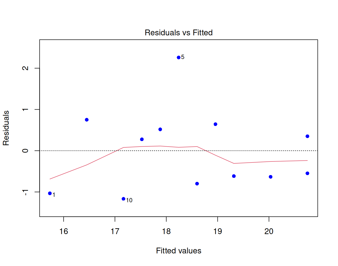
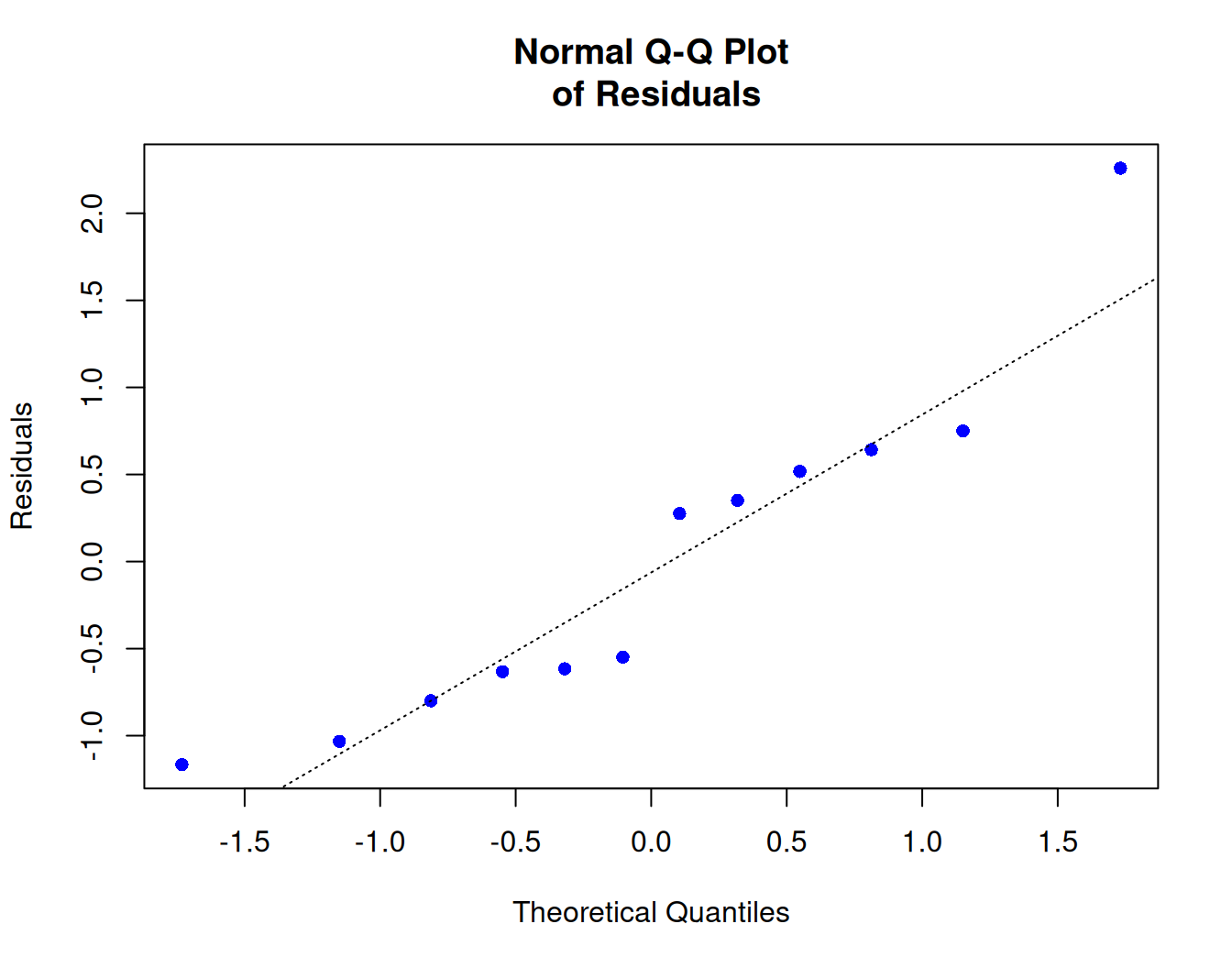
- Basic diagnostic plots for the simple linear regression straight line model (Figure 2)
lm(weight_gain ~ lysine_ingested, data = ex11_57);
Use (where possible) the R/R Commander output to answer the following questions:
a. Mention the symbol of the coefficient of determination and read from the R/R Commander output the estimated value.
b. Give an interpretation for the estimated coefficient of determinination in terms of the actual situation.
c. Explain why the coefficient of determination will increase when the sum of squares of the residuals decreases.
d. Determine the estimated correlation coefficient \(\rho\).
e. When calculated on the same data, will \(\mathbf{R}\) and \(\mathbf{r}\) always be exactly the same? Explain your answer.
f. Mention the assumptions for a simple linear regression straight line model.
g. Use (where possible) the R/R Commander output to check the model assumptions one by one. Mention what part of the output you have used for the different assumptions and explain why/why not the assumption holds.