Tutorial 8

Learning objectives

After this tutorial the student should be able to:

recognize a situation for which a paired sample \(t\)-test for population mean difference is applicable;
apply a paired sample \(t\)-test for population mean difference;
calculate and interpret a confidence interval for \(\mu_d\);
distinguish the paired sample \(t\)-test situation from the one sample and the independent sample \(t\)–test situation;
mention and is aware of some ethical issues concerning research findings;
determine the probability to get false positive or false negative research findings.

Pre-class activity

Watch:

‘Why Most Published Research Findings Are False’ (Duration: 14:50 min.)

The clip is linked on Brightspace.

Hypothesis testing and confidence interval for \(\mu_d\): one sample with paired observations

Read:

O&L 7^th Edition:
- paragraph 6.4 pp.325-329, or
O&L 6^th Edition:
- paragraph 6.4 pp.314-319.

In this paragraph the situation of one sample with paired observations is treated. Two variables are measured simultaneously on the same experimental units. This yields a single sample with paired observations, for example observations before and after a treatment or observations on married couples. To analyse the data of one sample with paired observations \((y_{11}, y_{21}), (y_{12}, y_{22}), \ldots ,(y_{1n}, y_{2n})\), we have to calculate the paired differences \(d_i = y_{1i} - y_{2i}\). For the differences \(d_i\ \forall\ i \in \{ 1, 2,\ldots,n\}\) we can apply the theory of the one sample situation.

Hypothesis testing for \(\mu_d\)

Definition \(\mu_d =\) (population) mean difference between\(\ldots\)

null hypothesis \(\mbox{H}_0:\ \mu_d = (\mu_d)_0\), where \((\mu_d)_0\) is a placeholder for a hypothesized value.
test statistic (T.S.): \(t = \frac{\bar{d} - (\mu_d)_0}{\mbox{SE}(\bar{d})} = \frac{\bar{d} - (\mu_d)_0}{s_d\ /\ \sqrt{n}}\)
Under \(\mbox{H}_0\) T.S. \(t\) follows a Student’s \(t\)-distribution with \(\nu = n - 1\) degrees of freedom.

etc.

Confidence interval for \(\mu_d\)

An unbiased estimator for \(\mu_d\) is \(\hat{\mu}_d = \bar{d}\) with standard error \(\mbox{SE}(\bar{d}) = s_d\ /\ \sqrt{n}\).
The limits of a \((1 - \alpha) \times 100\%\) confidence interval for \(\mu_d\) are \(\bar{d} \pm t_{\alpha/2} \times s_d / \sqrt{n}\), where \(t_{\alpha/2}\) comes from a Student’s \(t\)-distribution with \(\nu = n - 1\) degrees of freedom.

Some ethics concerning research findings

Some ethical issues concerning research findings are introduced and shortly discussed in class, to make you aware of these issues.

Exercises to be done during the tutorial

Exercise 8.1 up to and including Exercise 8.3 are in the presentation handouts of Tutorial 8. Check Brightspace for answers/feedback.

Exercise 8.1

a. Is the following experiment an example of 2 independent samples or paired observations?

In the United States of America an experiment was carried out to evaluate the effectiveness of a treatment against tapeworms in the stomach of sheep. Twenty-four infected sheep (of similar age and health), were randomly assigned, either to a control or a treatment group. After 6 months all sheep were slaughtered, and the number of tapeworms were counted.

b. Is the following experiment an example of 2 independent samples or paired observations?

A river may be contaminated by dispersion of zinc. Zinc possibly originates from the riverbed. Therefore, near the riverbed higher concentrations are expected. Zinc concentrations were measured at 6 locations, at the water surface of the river as well as near the riverbed.

Exercise 8.2

R/R Commander output useful for answering the questions:

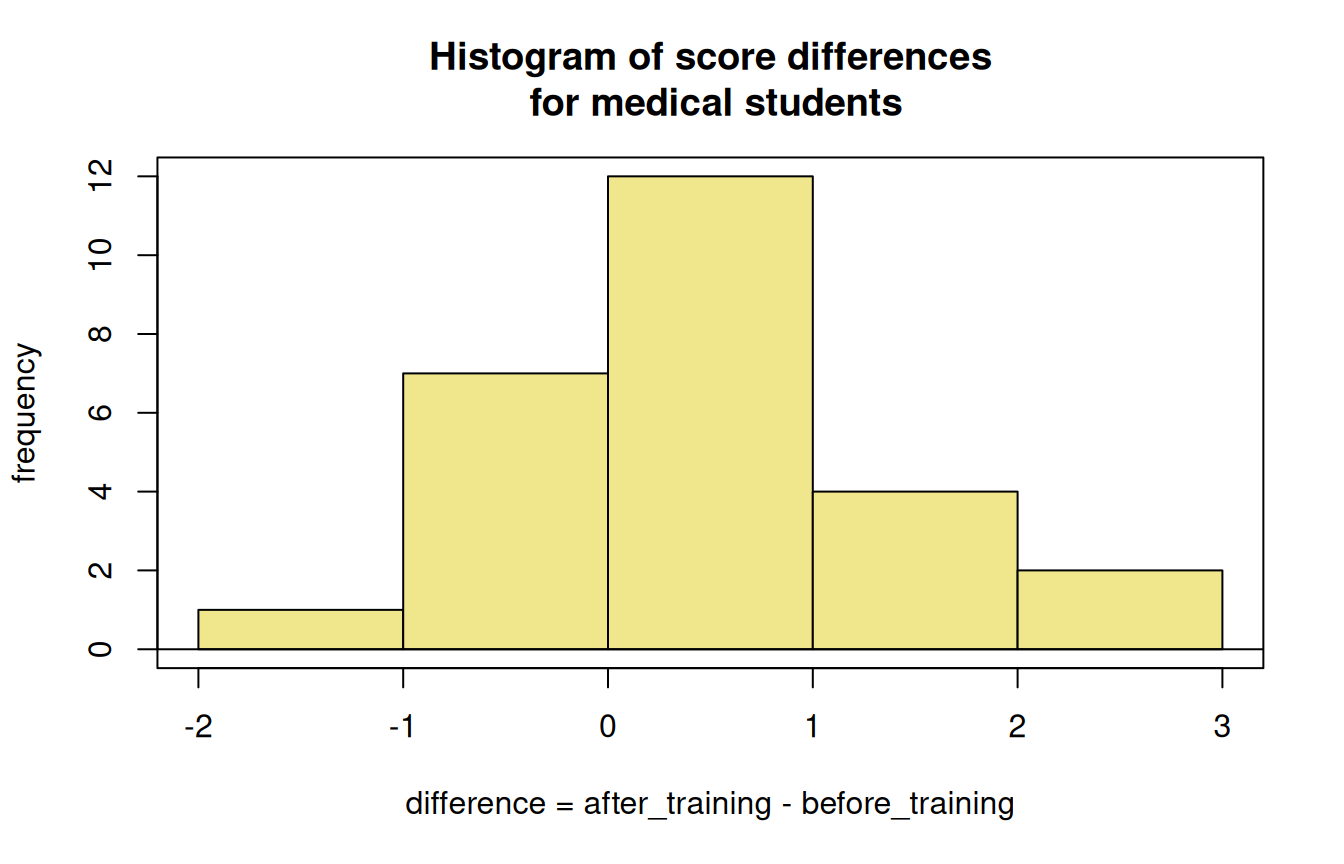
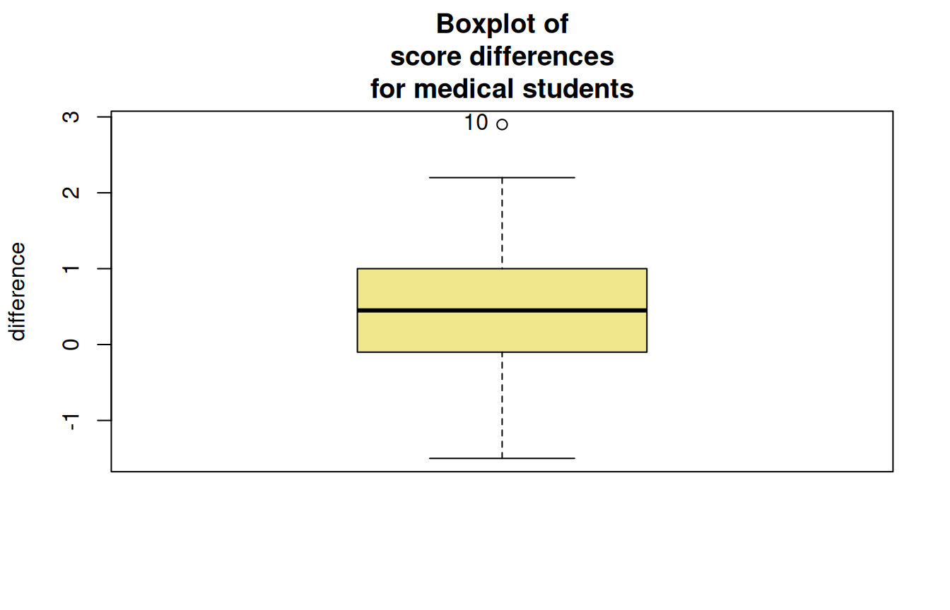
Numerical summaries of the medical students scores (see Table 1)

Table 1: Numerical summary of the medical students scores.

	mean	sd	se(mean)	n
after_training	7.14231	1.04045	0.20405	26
before_training	6.60385	1.29876	0.25471	26
difference	0.53846	0.94703	0.18573	26

Histogram (Figure 1 (a)) and boxplot (Figure 1 (b)) of the differences in scores after and before communication training for medical students.

Q-Q plot of score differences for medical students (Figure 2)

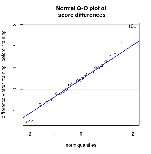
Figure 2: Q-Q plot of differences in scores after and before communication training for medical students.

a. Use hypothesis testing to investigate the research question: Does communication training improve the communication skills of medical students? Check the assumptions, use \(\alpha = 0.05\) and mention all steps.

b. Construct a 95% Confidence Interval for the (population) mean difference in scores after and before communication training for the medical students.

Exercise 8.3

Apart from ethical issues in research, there is a probability of wrong conclusions in research.

Suppose that at Wageningen University 550 hypotheses (550 different studies) are researched every year. From these 250 (alternative) hypotheses are true, 300 (alternative) hypotheses are not true. Probability Type I error = 0.05, Probability Type II error = 0.30. We assume correct research, and no publication bias.

Template for answering the questions:

Decision	\(\mbox{H}_0\) true	\(\mbox{H}_{\mbox{a}}\) true	Total
Reject \(\mbox{H}_0\)	\(P(\mbox{Type I Error}) = ?\)	Correct (TP)
	\(? \times \ldots = \ldots\) (FP)	\((1 - ??) \times \ldots = \ldots\)	\(\ldots\)
Do not reject \(\mbox{H}_0\)	Correct (TN)	\(P(\mbox{Type II Error}) = ??\)
	\((1 - ?) \times \ldots = \ldots\)	\(?? \times \ldots = \ldots\) (FN)	\(\ldots\)
Total	\(\ldots\)	\(\ldots\)	\(\ldots\)

In this table:

Reject \(\mbox{H}_0\), and \(\mbox{H}_{\mbox{a}}\) has been shown:
- When in reality \(\mbox{H}_0\) is true, there will be false positives (FP).
- When in reality \(\mbox{H}_{\mbox{a}}\) is true, there are true positives (TP).
Do not reject \(\mbox{H}_0\), and \(\mbox{H}_{\mbox{a}}\) has been not shown:
- When in reality \(\mbox{H}_0\) is true, there are true negatives (TN).
- When in reality \(\mbox{H}_{\mbox{a}}\) is true, there will be false negatives (FN).

Calculate:

the percentage of wrong conclusions of all the conclusions where \(\mbox{H}_0\) is rejected, and \(\mbox{H}_{\mbox{a}}\) has been shown.
the percentage of correct conclusions (i.e., \(\mbox{H}_{\mbox{a}}\) correctly shown or correctly not shown).

Post-class activity

Watch:

‘Why Most Published Research Findings Are False’ (Duration: 14:50 min.), when not done as pre-class activity,
‘How to distinguish a two independent samples situation from a paired sampled situation.’ (Duration: 7:15 min.)

All of the clips are linked on Brightspace.

Exercises to be done after the tutorial

For answers/feedback check Brightspace.

Exercise 8.4

Do either

Exercise 6.28ac O&L 7^th Edition p.351, or
Exercise 6.28ac O&L 6^th Edition p.342

R/R Commander output useful for answering the questions:

Numerical summary for the SENS values (Table 2).

Table 2: Numerical summary for the SENS values.

	mean	sd	se(mean)	n
after	5.402	5.155896	1.630437	10
before	7.986	8.123847	2.568986	10
difference	2.584	9.490733	3.001233	10

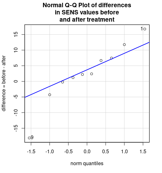
Q-Q Plot of the differences in SENS values before and after treatment (Figure 3).

Figure 3: Q-Q Plot of the differences in SENS values before and after treatment.

One-tailed Paired t-test:
- data: before and after
- \(t =\) 0.86098, df = 9, p-value = 0.2058
- alternative hypothesis: true mean difference is greater than 0
- 95 percent confidence interval: (-2.9175993, )
- sample estimates:
  - mean difference: \(2.584\)

Exercise 8.5

Do either

Exercise 6.57 O&L 7^th Edition p.359, or
Exercise 6.57 O&L 6^th Edition p.351

Additional questions

Which of the plots (Figure 4) is used to check whether the assumption of normality is met?

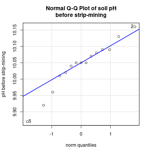
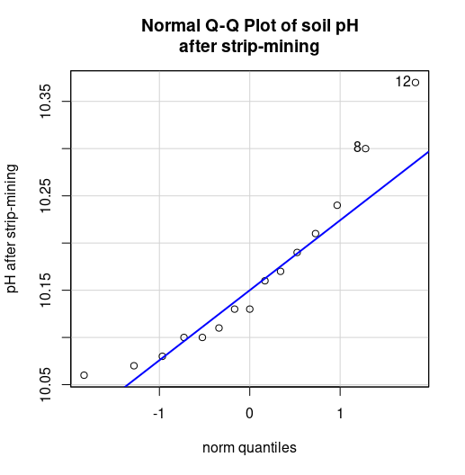
Provide arguments and draw your conclusion with respect to this assumption.

Answer the questions in the following order: b., a., c., d., Additional question I, Additional question II. Use \(\alpha = 0.01\).

R/R Commander output useful for answering the questions:

Left-tailed Paired t-test:
- data: before and after
- \(t =\) -4.45283, df = 14, p-value = 2.7^{-4}
- alternative hypothesis: true mean difference is less than 0
- 99 percent confidence interval: (-, -0.0500933)
- sample estimates:
  - mean difference: \(-0.122\)

Right-tailed Paired t-test:
- data: before and after
- \(t =\) -4.45283, df = 14, p-value = 0.99973
- alternative hypothesis: true mean difference is greater than 0
- 99 percent confidence interval: (-0.1939067, )
- sample estimates:
  - mean difference: \(-0.122\)

Two-tailed Paired t-test:
- data: before and after
- \(t =\) -4.45283, df = 14, p-value = 5.5^{-4}
- alternative hypothesis: true mean difference is not equal to 0
- 99 percent confidence interval: (-0.2035604, -0.0404396)
- sample estimates:
  - mean difference: \(-0.122\)

Exercise 8.6

Do either

Exercise 6.58 O&L 7^th Edition p.359, or
Exercise 6.58 O&L 6^th Edition p.351

Provide a reasoning for your chosen answer.

Exercise 8.7

In a large German university 1500 research hypothesis were tested in the past year. Assume that 400 alternative hypotheses are true. Furthermore assume the probability of a Type I Error to be \(0.05\) and the probability of a Type II Error to be \(0.30\).

a. Determine how many of the studies may have a false negative.

b. What is the percentage of false negatives?

c. And what is the percentage of false positives?

d. What will happen with the percentage false positives, when the probability of a Type I Error would be 0.01 instead of 0.05?