Tutorial 6

Learning outcomes

After this tutorial the student should be able to:

explain and interpret the general concepts of hypothesis testing: \(\mbox{H}_0\), \(\mbox{H}_{\mbox{a}}\), test statistic, \(\alpha\);
explain and interpret the concept of a p-value;
mention the eight steps of hypothesis testing using a p-value;
mention the eight steps of hypothesis testing using a Rejection Region;
apply a test for a population mean \(\mu\) for the one sample situation using a p-value;
apply a test for a population mean \(\mu\) for the one sample situation using a Rejection Region.

Pre-class activity

Watch:

‘Statistics, Student’s t-distribution, Gosset, and Guinness’ (Duration: 2:49 min.)

The clip is linked on Brightspace.

Hypothesis testing

In this tutorial hypothesis testing will be introduced.

In the next section the concepts related to hypothesis testing are given (see first box) and the general idea of hypothesis testing is discussed. Afterwards the level of significance (= p-value) is introduced and in the subsequent section the eight steps of hypothesis testing with the p-value are given. Additionally this is applied to a hypothesis about the population mean \(\mu\): the one-sample t-test. The theoretical part is illustrated with an example including the R/R Commander output of the one-sample \(t\)-test.

In the concluding section of this tutorial the eight steps of hypothesis testing using the rejection region (R.R.) are given. This is followed up by an example using the same data as before and applying a one-sample t-test again to illustrate, that using the R.R. is just another way to answer your research question.

Read:

O&L 7^th Edition:
- paragraph 5.4 pp.242-249 to the end of example 5.7, or
O&L 6^th Edition:
- paragraph 5.4 pp.232-239 to the end of example 5.7.

General concepts of hypothesis testing

concept	description
null hypothesis \(\mbox{H}_0\)	the hypothesis to be tested, which is rejected or not rejected
alternative hypothesis (\(\mbox{H}_{\mbox{a}}\), or \(\mbox{H}_1\))	the research hypothesis, which may or may not be proven based on the random sample
test statistic	a function of the observations, which is used for testing \(\mbox{H}_a\) (test statistic is often abbreviated as T.S.)
type I error	\(\mbox{H}_0\) is rejected, while \(\mbox{H}_0\) is true (see Tutorial 7)
type II error	\(\mbox{H}_0\) is not rejected, while \(\mbox{H}_{\mbox{a}}\) is true (see in Tutorial 7)
\(\alpha\) (significance level)	maximum probability allowing a type I error
p-value or level of significance	the observed p-value is the probability to find the observed outcome or a more extreme outcome for the test statistic, given that the null hypothesis is true
	if p-value > \(\alpha\) then \(\mbox{H}_0\) is not rejected and \(\mbox{H}_{\mbox{a}}\) is not shown/not accepted
	if p-value \(\leq \alpha\) then \(\mbox{H}_0\) is rejected and \(\mbox{H}_{\mbox{a}}\) is shown/accepted
rejection region	a collection of all possible values of the test statistic for which \(\mbox{H}_0\) has to be rejected (rejection region is often abbreviated as R.R.)

Please note that any hypothesis test can be conducted by using a p-value or by using a rejection region. In scientific papers, almost always a p-value is used. There is an ongoing discussion about the advantages and disadvantages of the p-value.

The level of significance (p-value) of a test

Read:

O&L 7^th Edition:
- paragraph 5.6 pp.257-260, or
O&L 6^th Edition:
- paragraph 5.6 pp.246-249.

Test procedure in eight steps using the p-value

When testing with a test statistic, and a p-value mention:

Definition of the parameter(s)!

the null-hypothesis \(\mbox{H}_0\) versus the alternative hypothesis \(\mbox{H}_{\mbox{a}}\)
the test statistic (T.S.)
the distribution of the test statistic under \(\mbox{H}_0\)
the behavior of the test statistic under \(\mbox{H}_{\mbox{a}}\) (i.e., “higher”/“lower”/“higher or lower” values than under \(\mbox{H}_0\))
the type (right-, left-, two-tailed) p-value
the outcome of the test statistic based on the observations
the level of significance (p-value)
the conclusion:
- when p-value \(\leq \alpha\) then \(\mbox{H}_0\) is rejected and \(\mbox{H}_{\mbox{a}}\) is shown;
- when p-value \(> \alpha\) then \(\mbox{H}_0\) is not rejected and \(\mbox{H}_{\mbox{a}}\) is not shown.
  Formulate the conclusion in words with respect to the research question (in terms of \(\mbox{H}_{\mbox{a}}\)).

Remarks about the hypothesis testing procedure steps.

The book O&L uses \(5\) steps instead of \(8\) steps. See O&L 7^th Edition p.243, or O&L 6^th Edition p.233. In the tutorials, and Lecture Notes (examples and exercises) the eight steps are used to provide a more clear overview and understanding.

With respect to the \(8\) steps in the hypothesis testing procedure:

The first five steps (of the eight) need to be written down before collecting (and analyzing) the data
The collected data will be used only in step \(6\) and onwards!
The null distribution of the test statistic is the distribution of the test statistic, assuming the null hypothesis to be true.

One-sample t-test: hypothesis testing for a population mean \(\mu\)

The one-sample t-test is applied to, as the name suggests, a single simple random sample, in which the variable (e.g., \(y\)) is continuous quantitative.

Hypothesis testing for \(\mu\): the one-sample t-test

Definition: \(\mu =\) (population) mean\(\ldots\)

null hypothesis \(\mbox{H}_0:\ \mu \leq \mu_0\), or \(\mu \geq \mu_0\), or \(\mu = \mu_0\) (\(\mu_0\) is a placeholder for the hypothesized value)
Test Statistic (T.S.): \(t = \frac{\bar{y} - \mu_0}{\mbox{SE}(\bar{y})} = \frac{\bar{y} - \mu_0}{s\ /\ \sqrt{n}}\)
Under \(\mbox{H}_0\) T.S. \(t\) follows a Student’s \(t\)-distribution with \(\nu = n - 1\) degrees of freedom etc.

Example 6.1

A lecturer claims that students can do the exam of his course within two hours. For this reason he wants to shorten the exam time from \(3\) to \(2\) hours in the coming academic year. The student board doubts the claim of the lecturer and thinks that it takes more than two hours to complete the exam. To show that the student board is right, a student asked \(25\) random students who took the exam recently, how much time in minutes \(y\) it took them to complete the exam. Test (\(\alpha = 0.05\)) whether the student board is right. Use the output below for step \(6\) – \(8\). You may assume that the \(25\) observations are independent and normally distributed with \(\mbox{E}(y) = \mu\).

Solution:
Before starting the actual test procedure, formulate the research question (RQ), define the parameter of interest, and decide (based on the available information) which test is the most appropriate.

RQ: Is the expected value in the population for the time to complete the exam more than \(120\) minutes?
Parameter of interest: \(\mu\): population mean time in minutes to complete the exam

Available information: There is one random sample of \(25\) students (\(n = 25\)); the variable \(y\) is the time in minutes to complete the exam; \(\sigma\) is not mentioned and hence its value is unknown; \(y\) is normally distributed; the research question is about the population mean \(\mu\) (expected value). From the combination of these facts we know that we may apply a one-sample \(t\)-test.

\(\mbox{H}_0:\ \mu \leq 120\) versus \(\mbox{H}_{\mbox{a}}:\ \mu > 120\)
The test statistic (T.S.): \(t = \frac{\bar{y} - \mu_0}{s\ /\ \sqrt{n}} = \frac{\bar{y} - 120}{s\ /\ \sqrt{25}}\)
Under \(\mbox{H}_0\) T.S. \(t\) follows a \(t\)-distribution with \(\nu = n - 1 = 24\) degrees of freedom.
Under \(\mbox{H}_{\mbox{a}}\) T.S. \(t\) tends to higher values than under \(\mbox{H}_0\).
The p-value is right-tailed.

This is what can be stated without using the data set itself. The data (see Table 1) as well as the output from a one-sample \(t\)-test is shown below.

Table 1: Time in minutes needed by \(25\) students to complete the exam.

170.4767	132.8770	184.02669	146.67294	104.78553
178.4164	115.8079	133.20909	164.94575	157.45583
138.8814	125.9051	99.87364	90.46134	144.35779
139.3965	113.2711	123.57045	182.56808	86.37873
158.9425	108.8226	121.47880	104.32277	126.86655

t.test(examtime_min, alternative = "greater", mu = 120, conf.level = 0.95)

#> 
#>  One Sample t-test
#> 
#> data:  examtime_min
#> t = 2.485, df = 24, p-value = 0.01016
#> alternative hypothesis: true mean is greater than 120
#> 95 percent confidence interval:
#>  124.4084      Inf
#> sample estimates:
#> mean of x 
#>  134.1509

Outcome T.S.: \(t = \frac{\bar{y} - 120}{s\ /\ \sqrt{25}} \approx 2.485\) (from output above).
p-value: \(P(t \geq 2.485) \approx 0.0102\) (In general, p-values are reported with 4 decimals.)
\(p\mbox{-value}\approx 0.0102 < 0.05\). Therefore, \(\mbox{H}_0\) is rejected, \(\mbox{H}_{\mbox{a}}\) has been shown. It is shown (with \(\alpha = 0.05\)) that the expected time to complete the exam is more than two hours.

Test procedure in eight steps using the rejection region

When testing with a test statistic, and a rejection region mention:

Definition of the parameter(s)!

the null hypothesis \(\mbox{H}_0\) versus the alternative hypothesis \(\mbox{H}_{\mbox{a}}\)
the test statistic (T.S.)
the distribution of the test statistic under \(\mbox{H}_0\)
the behavior of the test statistic under \(\mbox{H}_{\mbox{a}}\) (i.e., “higher”/“lower”/“higher or lower” values than under \(\mbox{H}_0\))
the type (right-, left-, two-tailed) rejection region (R.R.)
the outcome of the test statistic based on the observations
the rejection region (R.R.)
the conclusion:
- when the outcome of the T.S. is in the rejection region (R.R.) then \(\mbox{H}_0\) is rejected and \(\mbox{H}_{\mbox{a}}\) is shown;
- when the outcome of the T.S. is not in the rejection region (R.R.) then \(\mbox{H}_0\) is not rejected and \(\mbox{H}_{\mbox{a}}\) is not shown.
  Formulate the conclusion in words with respect to research question (in terms of \(\mbox{H}_{\mbox{a}}\)).

Example 6.2

For the description of the study as well as the research question please see Example 6.1.

Here additionally assume that there is not a computer at hand nor a graphing calculator. Therefore, finding the exact p-value is impossible and the rejection region needs to be used to perform the hypothesis test.

Solution:

\(\mbox{H}_0:\ \mu \leq 120\) versus \(\mbox{H}_{\mbox{a}}:\ \mu > 120\)
The test statistic (T.S.): \(t = \frac{\bar{y} - \mu_0}{s\ /\ \sqrt{n}} = \frac{\bar{y} - 120}{s\ /\ \sqrt{25}}\)
Under \(\mbox{H}_0\) T.S. \(t\) follows a \(t\)-distribution with \(\nu = 24\) degrees of freedom.
Under \(\mbox{H}_{\mbox{a}}\) T.S. \(t\) tends to higher values than under \(\mbox{H}_0\).
The rejection region (R.R.) is right-tailed.

This is what can be stated without using the data set itself.

The sample mean \(\bar{y}\) and the standard deviation \(s\) based on the data (see Table 1) shown above can be calculated:

mean(examtime_min)

#> [1] 134.1509

sd(examtime_min)

#> [1] 28.47202

Outcome T.S.: \(t = \frac{\bar{y} - 120}{s\ /\ \sqrt{25}} \approx \frac{134.1509 - 120}{28.472\ /\ 5} \approx 2.485\)
R.R.: \(t \geq 1.711\) (from O&L Table 2 with \(\alpha = 0.05\) and \(\nu = n - 1 = 25 - 1 = 24\) degrees of freedom)
The test statistic (\(t \approx 2.485\)) is in the rejection region. Therefore, reject \(\mbox{H}_0\), and \(\mbox{H}_{\mbox{a}}\) is shown.
It is shown (with \(\alpha = 0.05\)) that the expected time to complete the exam is more than two hours.

Exercises to be done during the tutorial

Exercise 6.1 is in the presentation handouts of Tutorial 6. For answers/feedback check Brightspace.

Post-class activity

Watch:

‘Statistics, Student’s t-distribution, Gosset, and Guinness’ (Duration: 2:49 min.), when not done as pre-class activity,
‘Understanding the p-value’ (Duration: 4:42 min.),
‘The Rejection Region’ (Duration: 7:29 min.).

All of the clips are linked on Brightspace.

Exercises to be done after the tutorial

For answers/feedback check Brightspace.

Exercise 6.2

The information as given with Exercise 5.3 is repeated here:
A factory delivers packages of sugar. A shop owner suspects that the weight of these packages is systematically less than 1000 g.

To prove this, the shop owner takes a random sample of 30 packages and weighs each package individually. The observed weights are denoted by \(y_1, y_2,\ldots,y_{30}\). The 30 observed weights can be considered as independent and normally distributed with \(\mbox{E}(y) = \mu\) and \(\sqrt{\mbox{var}(y)} = \sqrt{\sigma^2_y} = \sigma\).

Computational results: sample mean \(\bar{y} = 998.62\) g and sample standard deviation \(s = 5\) g.

a. Formulate the research question.

b. What is the appropriate test given the situation and the research question?

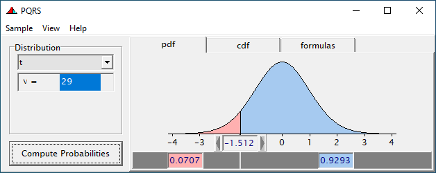
c. Apply the in b. mentioned test, to test the hypothesis of the shop owner (\(\alpha = 0.05\)). Write down all eight steps. Use Figure 1 to determine the p-value.

Figure 1: PQRS screenshot to determine the p-value.

d. Suppose you misunderstood the shop owner, who actually asked you to analyse the data with \(\alpha = 0.10\). Mention the step(s) of the analysis you should perform again to get the correct result.

e. Perform the step(s) you gave as an answer to d. for \(\alpha = 0.10\).

f. Without the PQRS screenshot in Figure 1, or a graphing calculator it would be impossible to determine the p-value. To answer the research question the rejection region must be used. Determine the rejection region (\(\alpha = 0.10\)) and draw the conclusion based on this rejection region.

Exercise 6.3

Do either

Exercise 5.42ab O&L 7^th Edition p.292, or
Exercise 5.44ab O&L 6^th Edition pp.282-283.

Notes to Exercise 6.3

Question a. is asking you to apply the appropriate test. Write down all eight steps and use for steps 6.–8. the R output below.

There is output for two different one-sample \(t\)-tests. Think carefully, which output is needed for hypothesis testing and which one is needed to read the confidence interval for \(\mu\).

With respect to Question b. first calculate the limits of the asked CI yourself, next check your answer using the R output.

R/R Commander output hypothesis tests for Exercise 6.3:

One-tailed hypothesis test:

#> 
#>  One Sample t-test
#> 
#> data:  volume
#> t = 3.6442, df = 17, p-value = 0.001003
#> alternative hypothesis: true mean is greater than 1600
#> 95 percent confidence interval:
#>  1661.845      Inf
#> sample estimates:
#> mean of x 
#>  1718.333

Two-tailed hypothesis test:

#> 
#>  One Sample t-test
#> 
#> data:  volume
#> t = 3.6442, df = 17, p-value = 0.002007
#> alternative hypothesis: true mean is not equal to 1600
#> 95 percent confidence interval:
#>  1649.824 1786.843
#> sample estimates:
#> mean of x 
#>  1718.333

Exercise 6.4

Refers to Exercise 6.3. Again perform the one-sample \(t\)-test, but now by using the rejection region approach.