Tutorial 7

Learning outcomes

After this tutorial the student should be able to:

explain Type I and Type II Error;
explain the effect of changing \(\alpha\) on the probability that a Type I Error occurs;
recognize a situation for which an independent samples \(t\)-test for difference between two population means is applicable;
apply an independent samples \(t\)-test for difference between two population means when \(\sigma_1^2 = \sigma_2^2\), as well as when \(\sigma_1^2 \neq \sigma_2^2\);
tell how \(\sigma_1^2 = \sigma_2^2\) is tested, and can act accordingly the outcome of this test with respect testing \(\mu_1 - \mu_2\);
calculate and interpret a confidence interval for \(\mu_1 - \mu_2\) when \(\sigma_1^2 = \sigma_2^2\), as well as when \(\sigma_1^2 \neq \sigma_2^2\);
distinguish the one sample \(t\)–test situation from the independent samples \(t\)–test situation.

Pre-class activity

Watch:

‘False Positives, False Negatives & Type I & II Errors’ (Duration: 2:29 min.)

The clip is linked on Brightspace.

Type I Error and Type II Error

Whenever a hypothesis test is applied, and a decision with respect to the null and alternative hypothesis has been taken based on the outcome of the test, there is a possibility that an error is made. Two types of error can be distinguished: The Type I and the Type II Error. In the mentioned paragraphs both types are explained.

(Re-)Read:

O&L 7^th Edition:
- paragraph 5.4 p.244 just above definitions 5.1 and 5.2 to p.246 Example 5.5, or
O&L 6^th Edition:
- paragraph 5.4 p.234 under Figure 5.5 to p.236 Example 5.5.

Confidence Interval and Hypothesis testing for \(\mu_1 - \mu_2\)

Read:

O&L 7^th Edition:
- paragraph 6.2 pp.303-315, or
O&L 6^th Edition:
- paragraph 6.2 pp.293-305.

This paragraph focuses on the situation of two independent samples. Therefore, one simple random sample with observations \(y_{11},\ y_{12},\ldots,\ y_{1n_1}\) with \(\mbox{E}(y_{1i}) = \mu_1\) and \(\mbox{var}(y_{1i}) = \sigma_1^2\ \forall\ i \in \{1,\ 2,\ldots ,\ n_1\}\) and a second simple random sample with observations \(y_{21},\ y_{22},\ldots,\ y_{2n_2}\) with \(\mbox{E}(y_{2i}) = \mu_2\) and \(\mbox{var}(y_{2i}) = \sigma_2^2\ \forall\ i \in \{1,\ 2,\ldots,\ n_2\}\).

Assume that both sets of observations within each sample are independent and normally distributed. Both samples are also considered to be independent from each other. The difference \(\mu_1 - \mu_2\) is estimated, the construction of a Confidence Interval, and the testing of the hypotheses for this difference are treated.

Confidence interval for \(\mu_1 - \mu_2\)

\(\sigma_1^2\) and \(\sigma_2^2\) are not assumed to be equal, i.e., \(\sigma_1^2 \neq \sigma_2^2\):
- an unbiased estimator for \(\mu_1 - \mu_2\) is \(\hat{\mu}_1 - \hat{\mu}_2 = \bar{y}_1 - \bar{y}_2\) with standard error: \[\mbox{SE}(\bar{y}_1 - \bar{y}_2) = \sqrt{\frac{s_1^2}{n_1} + \frac{s_2^2}{n_2}}\]
- the boundaries of a \((1 - \alpha) \times 100\%\) Confidence Interval for \(\mu_1 - \mu_2\) are given by: \[(\bar{y}_1 - \bar{y}_2) \pm t_{\alpha/2} \times \sqrt{\frac{s_1^2}{n_1} + \frac{s_2^2}{n_2}}\] where \(t_{\alpha/2}\) comes from a \(t\)-distribution with the degrees of freedom provided by the R/R Commander output.
\(\sigma_1^2\) and \(\sigma_2^2\) are assumed to be equal, i.e., \(\sigma_1^2 = \sigma_2^2 = \sigma^2\):
- an unbiased estimator for \(\mu_1 - \mu_2\) is \(\hat{\mu}_1 - \hat{\mu}_2 = \bar{y}_1 - \bar{y}_2\) with standard error: \[\mbox{SE}(\bar{y}_1 - \bar{y}_2) = \sqrt{s_p^2 \times \left(\frac{1}{n_1} + \frac{1}{n_2}\right)} = s_p \times \sqrt{\frac{1}{n_1} + \frac{1}{n_2}}\] where \(s_p^2\) is the pooled variance (an estimator for \(\sigma^2\)) and calculated as: \[s_p^2 = \frac{(n_1 - 1) \times s_1^2 + (n_2 - 1)\times s_2^2}{n_1 + n_2 - 2}\]
- the boundaries of a \((1 - \alpha) \times 100\%\) Confidence Interval for \(\mu_1 - \mu_2\) are given by: \[(\bar{y}_1 - \bar{y}_2) \pm t_{\alpha/2} \times \sqrt{s_p^2 \times \left(\frac{1}{n_1} + \frac{1}{n_2}\right)}\] where \(t_{\alpha/2}\) comes from a Student \(t\)-distribution with \(\nu = n_1 + n_2 - 2\) degrees of freedom.

Hypothesis testing for \(\mu_1 - \mu_2\)

\(\sigma_1^2\) and \(\sigma_2^2\) are not assumed to be equal, i.e., \(\sigma_1^2 \neq \sigma_2^2\):
- Null hypothesis \(\mbox{H}_0:\ \mu_1 - \mu_2 \leq D_0\), or \(\mu_1 - \mu_2 \geq D_0\), or \(\mu_1 - \mu_2 = D_0\)
- Test statistic (T.S.): \(t = \frac{(\bar{y}_1 - \bar{y}_2) - D_0}{\mbox{SE}(\bar{y}_1 - \bar{y}_2)} = \frac{(\bar{y}_1 - \bar{y}_2) - D_0}{\sqrt{\frac{s_1^2}{n_1} + \frac{s_2^2}{n_2}}}\)
- Under \(\mbox{H}_0\) T.S. \(t\) follows a \(t\)-distribution with \(\nu\) degrees of freedom, which can be read from the R/R Commander output.
\(\sigma_1^2\) and \(\sigma_2^2\) are assumed to be equal, i.e., \(\sigma_1^2 = \sigma_2^2 = \sigma^2\):
- Null hypothesis \(\mbox{H}_0:\ \mu_1 - \mu_2 \leq D_0\), or \(\mu_1 - \mu_2 \geq D_0\), or \(\mu_1 - \mu_2 = D_0\)
- Test statistic (T.S.): \(t = \frac{(\bar{y}_1 - \bar{y}_2) - D_0}{\mbox{SE}(\bar{y}_1 - \bar{y}_2)} = \frac{(\bar{y}_1 - \bar{y}_2) - D_0}{s_p \times \sqrt{\frac{1}{n_1} + \frac{1}{n_2}}}\)
- Under \(\mbox{H}_0\) T.S. \(t\) follows a Student \(t\)-distribution with \(\nu = n_1 + n_2 - 2\) degrees for freedom.

Remarks about equality or unequality of variances.

It is obvious that when \(\sigma_1^2 = \sigma_2^2\), also \(\sigma_1 = \sigma_2\) will hold. Generally this is referred to as the assumption of equal variances. To test whether this assumption holds, Levene’s test for equality of variance needs to applied before testing with an independent samples \(t\)-test. Levene’s test for equality of variance tests the hypotheses \(\mbox{H}_0:\ \sigma_1^2 = \sigma_2^2\) versus \(\mbox{H}_{\mbox{a}}:\ \sigma_1^2 \neq \sigma_2^2\). In the R/R Commander output the test statistic is given as a \(F\)-statistic and associated degrees of freedom. In this course this test statistic and degrees of freedom can be ignored. The only part of the output from Levene’s test, which requires interpretation is the p-value. This is given under Pr(>F) in the R/R Commander output for a Levene’s test:
- When this p-value is smaller than or equal to \(\alpha\), reject \(\mbox{H}_0:\ \sigma_1^2 = \sigma_2^2\) and \(\mbox{H}_{\mbox{a}}:\ \sigma_1^2 \neq \sigma_2^2\) has been shown. Perform the independent samples \(t\)-test under the assumption of unequal variances.
- When the p-value is larger than than \(\alpha\), do not reject \(\mbox{H}_0:\ \sigma_1^2 = \sigma_2^2\) and \(\mbox{H}_{\mbox{a}}:\ \sigma_1^2 \neq \sigma_2^2\) has not been shown. Perform the independent samples \(t\)-test under the assumption of equal variances.
When assuming unequal variances, the so-called Welch-Satterthwaite approximation for the degrees of freedom needs to be applied. This is discussed in O&L \(\mathbf{7}^{\mbox{th}}\) Edition pp.311-312, or O&L \(\mathbf{6}^{\mbox{th}}\) Edition pp.301-312. The details of the approximation for the degrees of freedom, can be skipped. They can be read from the R/R Commander output.

Exercises to be done during the tutorial

Exercise 7.1 is in the presentation handouts of Tutorial 7. For answers/feedback check Brightspace.

Exercise 7.1

The aim of this research into the effect of weasel scent on hamsters is to show that hamsters, that are exposed to weasel scent, have increased cortisol levels [ng/ml] in their blood.

Use the following notation:

\(\mu_A =\) the population mean cortisol level in hamsters not exposed to weasel scent, and
\(\mu_B =\) the population mean cortisol level in hamsters exposed to weasel scent.

Assume that the cortisol levels in both groups are normally distributed with means \(\mu_A\) and \(\mu_B\) and equal variance \(\sigma^2\).

Useful R/R Commander plots and output for answering the questions are given below.

Side-by-side boxplots (see Figure 1)

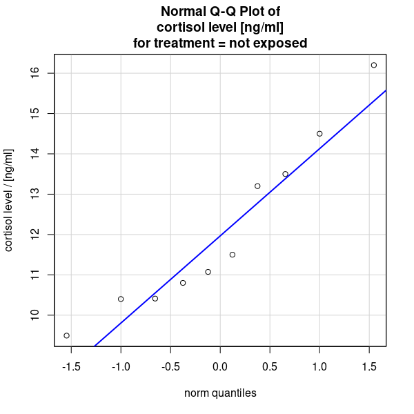
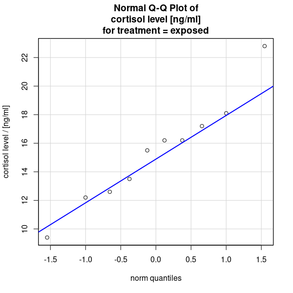
Figure 1: Side-by-side boxplots for the cortisol level [ng/ml] in hamsters not exposed, and exposed to weasel scent.

Q-Q Plots of cortisol level [ng/ml] in hamsters not exposed (see Figure 2 (a)), and exposed (see Figure 2 (b)) to weasel scent.

Numerical summary for the cortisol level [ng/ml] of hamsters not exposed and exposed to weasel scent (see Table 1)

Table 1: Numerical summary for the cortisol level [ng/ml] of hamsters not exposed and exposed to weasel scent.

	mean	sd	se(mean)	cortisol:n
not exposed	12.10773	2.144313	0.6780915	10
exposed	15.37000	3.715747	1.1750225	10

Levene’s test (see Table 2)

Table 2: Levene’s Test for Homogeneity of Variance (center = “mean”)

	Df	F value	Pr(>F)
group	1	1.4488	0.2443
	18

One-tailed Two Sample t-test:
- data: cortisol by treatment
- \(t =\) -2.4047, df = 18, p-value = 0.01358
- alternative hypothesis: true difference in means between group not exposed and group exposed is less than 0
- 95 percent confidence interval: (-, -0.9097619)
- sample estimates:
  - mean in group not exposed: \(12.10773\)
  - mean in group exposed: \(15.37\)

Two-tailed Two Sample t-test:
- data: cortisol by treatment
- \(t =\) -2.4047, df = 18, p-value = 0.02717
- alternative hypothesis: true difference in means between group not exposed and group exposed is not equal to 0
- 95 percent confidence interval: (-6.1124762, -0.4120652)
- sample estimates:
  - mean in group not exposed: \(12.10773\)
  - mean in group exposed: \(15.37\)

a. Check the assumption that the cortisol levels in both groups are normally distributed.

b. Compute the estimated difference between the parameters of interest (\(\mu_A - \mu_B\)).

c. The estimate of \(\sigma^2\) is 9.20. How is this value calculated based on the information given in the R/R Commander output?

d. Use answer c. to verify that the standard error of the estimator for \(\mu_A - \mu_B\) is approximately equal to \(1.3566\).

e. Verify whether it can be shown that the mean cortisol level in group B is higher than that in group A, at a significance level (\(\alpha\)) of \(0.05\). Give all 8 steps of the test.

f. Same question in e., but now use the Rejection Region approach instead.

g. Give the \(95\%\) confidence interval for the difference between the population means \(\mu_A - \mu_B\).

Post-class activity

Watch:

‘False Positives, False Negatives & Type I & II Errors’ (Duration: 2:29 min.), when not done as pre-class activity,
‘Levene’s test’ (Duration: 6:31 min.).

All of the clips are linked on Brightspace.

Exercises to be done after the tutorial

For answers/feedback check Brightspace.

Exercise 7.2

Do either

Exercise 5.16a O&L 7^th Edition p.288, or
Exercise 5.18a O&L 6^th Edition p.278

Additional question

Could you possibly have made a Type II Error in drawing your conclusion in question a. as specified above? Explain your answer.

Exercise 7.3

Read the research study about effects of an oil spill on plant growth:

O&L 7^th Edition pp.336-339, or
O&L 6^th Edition pp.325-328

Useful R/R Commander output for answering the questions of exercise 7.3:

Levene’s test (see Table 3)

Table 3: Levene’s Test for Homogeneity of Variance (center = “mean”)

	Df	F value	Pr(>F)
group	1	5.209	0.0252
	78

One-tailed Two Sample t-test:
- data: density by tract
- \(t =\) 3.8209, df = 78, p-value = 1.3^{-4}
- alternative hypothesis: true difference in means between group control and group oilspill is greater than 0
- 95 percent confidence interval: (6.5180789, )
- sample estimates:
  - mean in group control: \(38.475\)
  - mean in group oilspill: \(26.925\)

Two-tailed Two Sample t-test:
- data: density by tract
- \(t =\) 3.8209, df = 78, p-value = 2.7^{-4}
- alternative hypothesis: true difference in means between group control and group oilspill is not equal to 0
- 95 percent confidence interval: (5.5319554, 17.5680446)
- sample estimates:
  - mean in group control: \(38.475\)
  - mean in group oilspill: \(26.925\)

One-tailed Welch Two Sample t-test:
- data: density by tract
- \(t =\) 3.8209, df = 64.1027923, p-value = 1.5^{-4}
- alternative hypothesis: true difference in means between group control and group oilspill is greater than 0
- 95 percent confidence interval: (6.5049323, )
- sample estimates:
  - mean in group control: \(38.475\)
  - mean in group oilspill: \(26.925\)

Two-tailed Welch Two Sample t-test:
- data: density by tract
- \(t =\) 3.8209, df = 64.1027923, p-value = 3^{-4}
- alternative hypothesis: true difference in means between group control and group oilspill is not equal to 0
- 95 percent confidence interval: (5.5113368, 17.5886632)
- sample estimates:
  - mean in group control: \(38.475\)
  - mean in group oilspill: \(26.925\)

Perform the hypothesis test as described at O&L \(7^{\mbox{th}}\) Edition p.339 [O&L \(6^{\mbox{th}}\) Edition p.328] yourself following questions a., b., c. and d.

a. Formulate the research question (RQ), define the parameter(s) of interest and give arguments why the independent samples t-test is here the appropriate test.

b. Denote/write down the first five steps of the test procedure for the independent samples t-test.

c. Next use the appropriate part of the R/R Commander output, to test whether the variances can be assumed unequal or equal. Mention the null and alternative hypothesis for this test, the p-value, your conclusion in words, and whether the result implies that you need the Welch-Satterthwaite approximation for the degrees of freedom, when proceeding with the independent sample t-test.

d. Finally, use the appropriate output (see your answers to questions b. and c.) to continue with the independent samples t-test. Write down all steps (i.e., step 6., 7. and 8.).

e. Give the formula for the 95% Confidence Interval of the difference in (population) mean plant density between control and restored oilspill sites (see O&L p.341 [p.330 in the \(\mathbf{6}^{\mbox{th}}\) Edition]) and read the result from the appropriate R/R Commander output.

Exercise 7.4

Do either

Exercise 6.6ab O&L 7^th Edition p.345, or
Exercise 6.6ac O&L 6^th Edition p.334

Notes Exercise 6.6ab O&L 7^th Edition

Note to exercise 6.6a.: Start with formulating the research question (RQ), defining the parameter(s) of interest and mentioning the name of the correct hypothesis test. Next apply the hypothesis test and mention all the steps.

For the situation described, the interest is in the difference between two population means. This difference is denoted by \(D_0\) in the equation for the test statistic \(t\). Quite often this difference will be \(0\), and therefore, denoted as \(D_0 = 0\). However, in the given situation the hypothesis test described tests whether the difference in the (population) mean dissolved oxygen level between up- and downstream of a community is more than \(0.5\). R/R Commander will always test with \(D_0 = 0\). Therefore, the output from R/R Commander can not be used. The outcome of the test statistic \(t\) would have to be manually calculated and an exact p-value can not be obtained. The solution is to use the rejection region approach.

Though the output for the \(t\)-test can not be used in this particular case, R/R Commander can of course still be used to calculate sample means, variances, perform Levene’s test and make graphical representations.

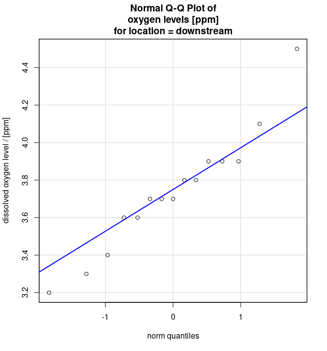
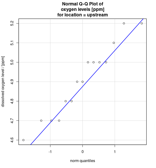
Note to exercise 6.6b.: Mention the plot(s) on which you based your answer.

R/R Commander output Exercise 6.6ab O&L 7^th Edition

Side-by-side boxplots (see Figure 3)

Figure 3: Side-by-side boxplots of dissolved oxygen levels [ppm] for locations up- and downstream from a riverside community.

Q-Q Plots of dissolved oxygen levels [ppm] for locations downstream (see Figure 4 (a)) and upstream (see Figure 4 (b)) from a riverside community.

(a) Downstream from a riverside community.

Levene’s test (see Table 4)

Table 4: Levene’s Test for Homogeneity of Variance (center = “mean”)

	Df	F value	Pr(>F)
group	1	1.5336	0.2259
	28

Numerical summary for the dissolved oxygen levels [ppm] in locations down- and upstream from a riverside community (see Table 5)

Table 5: Numerical summary for the dissolved oxygen levels [ppm] in locations down- and upstream from a riverside community.

	mean	sd	oxygen:n
downstream	3.740000	0.3202677	15
upstream	4.906667	0.1869556	15

Additional questions Exercise 6.6ab O&L 7^th Edition

I: Give the 99% Confidence Interval for the difference between the (population) mean dissolved oxygen level up- and downstream from a community.
II: Would a 95% Confidence Interval be wider or narrower than the 99% Confidence Interval? Provide argument to support your answer.
III: Suppose the 95% Confidence Interval was based on two samples of size 20. Would this change the confidence coefficient? Why or why not?

Notes Exercise 6.6ac O&L 6^th Edition

In the independent samples \(t\)-test R/R Commander uses an alphabetical order for the groups, when calculating the difference between group means. Therefore, in this question the difference is calculated as aboveTown - belowTown.

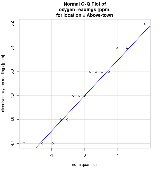
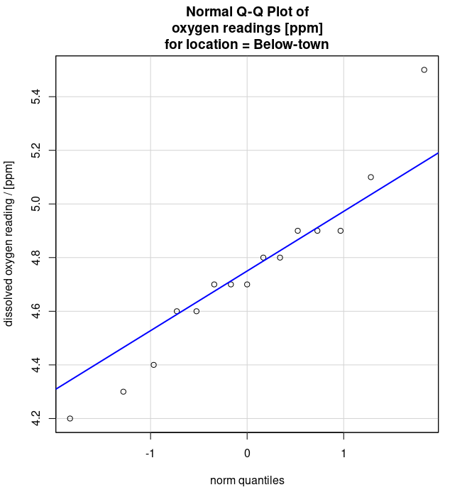
Note to exercise 6.6c.: Mention the plot(s) on which you based your answer.

R/R Commander output Exercise 6.6ac O&L 6^th Edition

Side-by-side boxplots (see Figure 5)

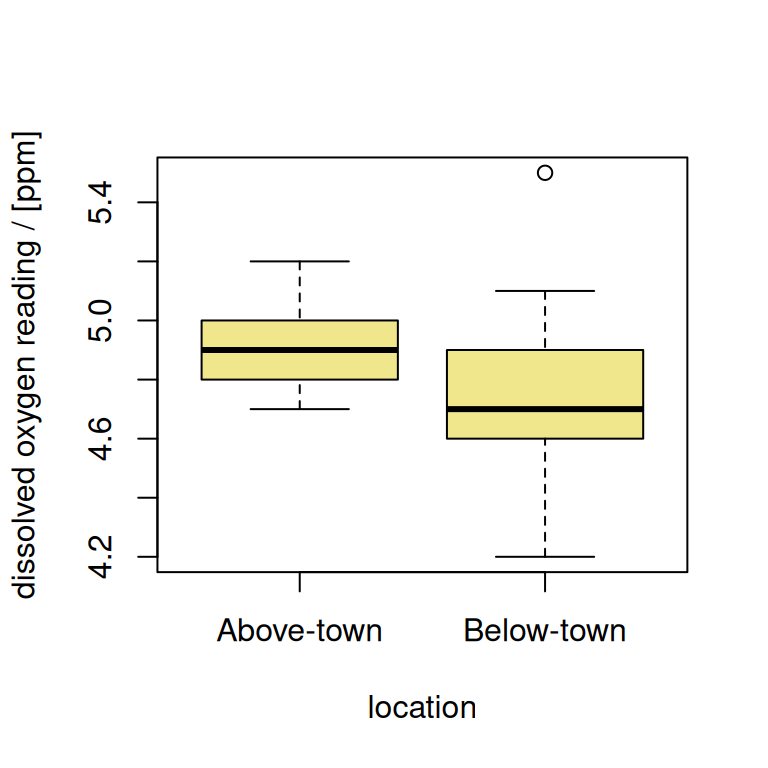
Figure 5: Side-by-side boxplots of dissolved oxygen readings [ppm] for locations above and below from a community town.

Q-Q Plots of dissolved oxygen readings [ppm] for locations above (see Figure 6 (a)) and below (see Figure 6 (b)) a community town.

Levene’s test (see Table 6)

Table 6: Levene’s Test for Homogeneity of Variance (center = “mean”)

	Df	F value	Pr(>F)
group	1	2.8932	0.1
	28

Two-tailed Two Sample t-test:
- data: oxygen by location
- \(t =\) 1.9551, df = 28, p-value = 0.06062
- alternative hypothesis: true difference in means between group Above-town and group Below-town is not equal to 0
- 95 percent confidence interval: (-0.0085891, 0.3685891)
- sample estimates:
  - mean in group Above-town: \(4.92\)
  - mean in group Below-town: \(4.74\)

Additional questions Exercise 6.6ac O&L 6^th Edition

I: Give the 95% Confidence Interval for the difference between the (population) mean dissolved oxygen level above and below a community town.
II: Would a 95% Confidence Interval be wider or narrower than the 99% Confidence Interval? Provide argument to support your answer.
III: Suppose the 95% Confidence Interval was based on two samples of size 20. Would this change the confidence coefficient? Why or why not?